Multiple Linear Regression
Jul 20, 2024
Introduction
Multiple linear regression is an extension of simple linear regression. It is used when we want to predict the value of a variable based on the value of two or more other variables. The variable we want to predict is called the dependent variable (or target variable). The variables we are using to predict the value of the dependent variable are called independent variables (or features).
# Import libraries

import numpy as np
import pandas as pd
import matplotlib.pyplot as plt
import seaborn as sns
Dataset
We will continue the kaggle dataset we used in the simple linear regression blog. The advertising budget is in thousands of dollars and the sales are in millions of dollars.
data = pd.read_csv('data/Advertising.csv', index_col=0)
data.head()| TV | Radio | Newspaper | Sales | |
|---|---|---|---|---|
| 1 | 230.1 | 37.8 | 69.2 | 22.1 |
| 2 | 44.5 | 39.3 | 45.1 | 10.4 |
| 3 | 17.2 | 45.9 | 69.3 | 9.3 |
| 4 | 151.5 | 41.3 | 58.5 | 18.5 |
| 5 | 180.8 | 10.8 | 58.4 | 12.9 |
Equation of Multiple Linear Regression
The general mathematical equation for multiple linear regression is:
$$
y = \beta_0 + \beta_1 x_1 + \beta_2 x_2 + \ldots + \beta_n x_n + \epsilon
$$
Where:
- $y$ is the dependent variable
- $x_1$, $x_2$, $\ldots$, $x_n$ are the independent variables
- $\beta_0$ is the Y-intercept
- $\beta_1$, $\beta_2$, $\ldots$, $\beta_n$ are the coefficients for the independent variables $x_1$, $x_2$, $\ldots$, $x_n$
- $\epsilon$ is the error term
The equation for our dataset will be:
$$
sales = \beta_0 + \beta_1 \times TV + \beta_2 \times radio + \beta_3 \times newspaper + \epsilon
$$
Components of a Linear Regression Equation
1. Dependent Variable ($y$)
The dependent variable is the variable we are trying to predict. It is the variable that we expect to change when we change the independent variables. In the context of multiple linear regression, $y$ regresents the value that we are trying to predict based on the values of $x_1$, $x_2$, $\ldots$, $x_n$. In the advertising dataset, the dependent variable is the sales revenue.
2. Independent Variables ($x_1$, $x_2$, $\ldots$, $x_n$)
The independent variables are the variables that we believe are influencing the value of the dependent variable. In multiple linear regression, there are two or more independent variables, each contributing to the prediction of the $y$ variable. In the context of the advertising dataset, the independent variables are TV, radio, and newspaper advertising budgets.
3. Intercept ($\beta_0$)
The intercept ($\beta_0$) is the value of $y$ when all independent variables are equal to zero. It is the value of $y$ when all independent variables have no effect on the dependent variable. In the context of the advertising dataset, the intercept represents the sales revenue when there is no advertising budget for TV, radio, or newspaper.
4. Coefficients ($\beta_1$, $\beta_2$, $\ldots$, $\beta_n$)
The coefficients represent the change in the dependent variable for a one-unit change in the corresponding independent variable, while holding all other independent variables constant. The coefficients tell us how much the dependent variable is expected to increase or decrease when that independent variable increases by one unit. In our example, consider the coefficient for the TV variable ($\beta_1$). If $\beta_1$ is 0.05, it means that for every additional $1000 spent on TV advertising, sales are expected to increase by 50 thousand dollars.
5. Error Term ($\epsilon$)
The error term represents the difference between the observed value of the dependent variable and the predicted value. It accounts for the variability in the dependent variable that is not explained by the independent variables. The goal of linear regression is to minimize the error term by finding the best-fitting line that explains the relationship between the dependent and independent variables.
Objectives
The objectives of multiple linear regression are to:
- Estimate the coefficients ($\beta_1$, $\beta_2$, $\ldots$, $\beta_n$)
- Evaluate the fit of the regression model.
- Make predictions based on the regression model.
- Understand the strength and direction of the relationships between the dependent variable and each independent variable.
Assumptions of Multiple Linear Regression
- Linearity: The relationship between the dependent variable and the independent variables is linear.
- Independence: The residuals (errors) are independent of each other.
- Homoscedasticity: The residuals have constant variance.
- Normality: The residuals are normally distributed.
- No multicollinearity: The independent variables are not highly correlated with each other.
We will conver the assumptions in more detail in the another blog.
Exploratory Data Analysis
We will do some exploratory data analysis to understand the relationship between the independent variables (TV, radio, newspaper) and the dependent variable (sales).
fig, axs = plt.subplots(1, 3, sharey=True, figsize=(15, 5))
colors = ['blue', 'green', 'red']

for ax, medium, color in zip(axs, data.columns[:-1], colors):
    data.plot(kind='scatter', x=medium, y='Sales', ax=ax, color=color)
    ax.set_title(f'Sales vs {medium}', fontsize=14)
    ax.set_ylabel('Sales', fontsize=12)
    ax.set_xlabel(medium, fontsize=12)
    ax.grid(True)

plt.tight_layout()
plt.show()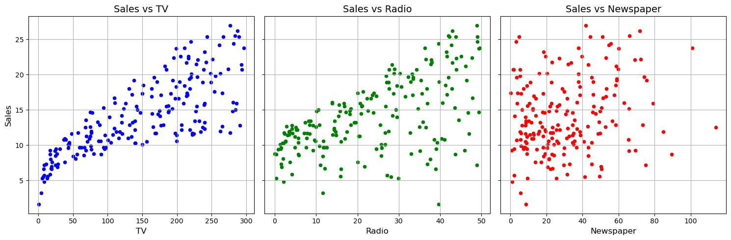
The plot above shows the clear positive relationship between the TV advertising budget and sales revenue. As the TV advertising budget increases, the sales revenue also increases. The relation also appears positive for radio advertising budget and sales revenue, but the relationship is not as strong as TV. The newspaper advertising budget does not show a clear relationship with sales revenue.
Data Preparation
Splitting the Data
We will split the data into training and testing sets. We will use the training set to train the model and the testing set to evaluate the model’s performance.
from sklearn.model_selection import train_test_split

X = data.drop('Sales', axis=1)
y = data['Sales']

X_train, X_test, y_train, y_test = train_test_split(X, y, test_size=0.2, random_state=42)
print(X_train.shape)
print(X_test.shape)
(160, 3)
(40, 3)
Scaling
In multiple linear regression, it is important to scale the data before fitting the model. Scaling the data ensures that all variables have the same scale and are on a similar range. This is important because the coefficients in the regression equation are sensitive to the scale of the variables. If the variables are on different scales, the coefficients will be on different scales as well, making it difficult to compare the importance of each variable.
from sklearn.preprocessing import StandardScaler

scaler = StandardScaler()
X_train_scaled = scaler.fit_transform(X_train)
X_test_scaled = scaler.transform(X_test)
Fitting the Model
from sklearn.linear_model import LinearRegression

model = LinearRegression()
model.fit(X_train, y_train)

# Get the slope and intercept of the line best fit.

print(f'The coefficient of the linear model is {model.coef_}')
print(f'The intercept of the linear model is {model.intercept_:.2f}')
The coefficient of the linear model is [0.04472952 0.18919505 0.00276111]
The intercept of the linear model is 2.98
coefficients = pd.DataFrame([model.coef_], columns=X.columns, index=['Coefficient'])
coefficients| TV | Radio | Newspaper | |
|---|---|---|---|
| Coefficient | 0.04473 | 0.189195 | 0.002761 |
Therefore, the equation of the best fit line is:
$$ \text{Sales} = 2.98 + 0.045 \times \text{TV} + 0.19 \times \text{Radio} - 0.003 \times \text{Newspaper} $$
Interpreting Results
- Intercept ($\beta_0$): The expected sales when all advertising budgets are zero. Therefore, if there is no advertising budget for TV, radio, or newspaper, the expected sales revenue is 2.98 million dollars.
- Coefficients ($\beta_1$, $\beta_2$, $\beta_3$): The coefficients represent the change in sales revenue for a one-unit change in the corresponding advertising budget, while holding all other advertising budgets constant. For example, the coefficient for TV advertising budget is 0.045. This means that for every additional $1000 spent on TV advertising, sales revenue is expected to increase by 45 thousand dollars.
Evaluating Model Performance
from sklearn.metrics import mean_squared_error, r2_score

y_pred = model.predict(X_test)

mse = mean_squared_error(y_test, y_pred)
r2 = r2_score(y_test, y_pred)

print(f"Mean Squared Error: {mse}")
print(f"R-squared: {r2}")
Mean Squared Error: 3.1740973539761046
R-squared: 0.899438024100912
Residual Analysis
The residual plot shows that the residuals are randomly distributed around zero, indicating that the model is capturing the underlying patterns in the data. The residuals are homoscedastic, meaning that the variance of the residuals is constant across all levels of the independent variables.
residuals = y_test - y_pred

plt.figure(figsize=(10, 5))
sns.histplot(residuals, kde=True, color='blue')
plt.title('Residuals Distribution', fontsize=16)
plt.xlabel('Residuals', fontsize=14)
plt.ylabel('Frequency', fontsize=14)
plt.grid(True)
plt.show()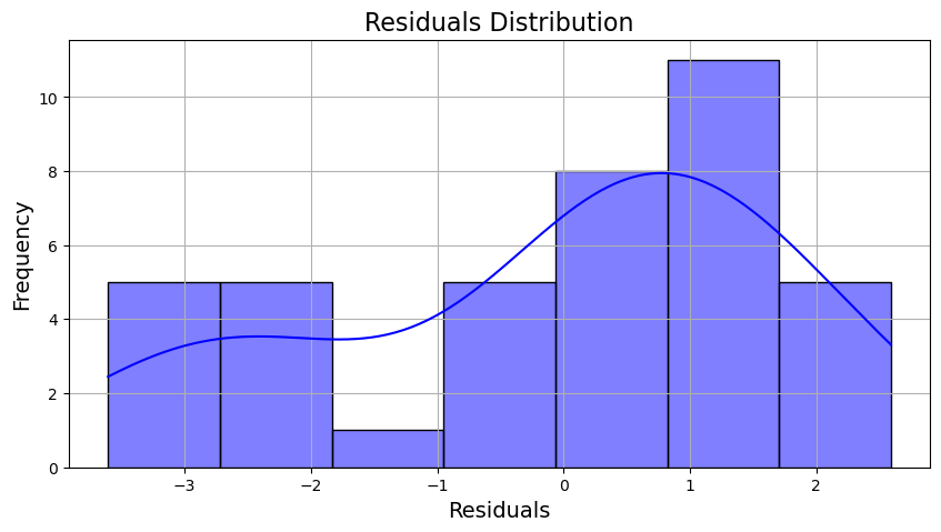
Conclusion
This analysis demonstrates how to perform multiple linear regression to predict sales revenue based on TV, radio, and newspaper advertising budgets. The model provides insights into the relationship between advertising budgets and sales revenue, allowing businesses to make data-driven decisions about their marketing strategies.
Key Findings
- TV Advertising: TV advertising has the strongest positive relationship with sales revenue. For every additional \$1000 spent on TV advertising, sales revenue is expected to increase by \$44,730. This suggests that TV advertising has positive returns on investment, although it is less cost-effective than radio advertising.
- Radio Advertising: Radio advertising also has a positive relationship with sales revenue, although the effect is smaller than TV advertising. For every additional \$1000 spent on radio advertising, sales revenue is expected to increase by \$189,195. This suggests that radio advertising can be an effective marketing channel for reaching a targeted audience.
- Newspaper Advertising: Newspaper advertising shows the least impact on sales revenue, with a coefficient of -0.003. This suggests that newspaper advertising may not be an effective marketing channel for driving sales revenue. Businesses may want to consider reallocating their advertising budgets from newspaper to TV or radio advertising to maximize sales revenue.
Deployment
The model can be deployed to make predictions on new data. By inputting the advertising budgets for TV, radio, and newspaper, the model can predict the expected sales revenue for a given set of advertising budgets. This information can help businesses optimize their marketing strategies and allocate resources effectively to maximize sales revenue.
For an interactive demonstration of the model, you can visit the Multiple Linear Regression Deployment. This applicaiton allows users to input the advertising budgets for TV, radio, and newspaper and see the predicted sales revenue based on the multiple linear regression model.
← Back to Blog