Simple Linear Regression
Jul 7, 2024
What is Linear Regression?
In simple words you try to predict value of one variable considering it have a linear relationship with other variable.
In linear regression you assume that value of one variable is dependent on the value of other variable. So when value of one variable increases or decreases, value of other variable also increases or decreases. Therefore, the relationship between the two variables is linear.
Regression is a statistical method used to predict the value of one variable based on the value of another variable. Linear regression is the most simple and commonly used regression model.
Let’s try to understand it with simple example.
I am using dataset from kaggle, which is a simple dataset of advertising data.
In this dataset, we have 4 columns: TV, Radio, Newspaper and Sales.
The TV, Radio and Newspaper columns are the amount of money spent on advertising on TV, Radio and Newspaper respectively. The Sales column is the amount of sales generated due to the advertising on TV, Radio and Newspaper.
For our understanding, we will consider TV as independent variable and Sales as dependent variable. We will try to predict the Sales based on the amount of money spent on TV advertising.
Hypothesis of Linear Regression
The hypothesis of linear regression is that the dependent variable is a linear combination of the independent variables.
For our example, the hypothesis is that the Sales is directly proportional to the amount of money spent on TV advertising.
The hypothesis can be represented as follows:
$$Sales = \beta_0 + \beta_1 * TV$$
Where:
- Sales is the dependent variable
- TV is the independent variable
- $\beta_0$ is the intercept
- $\beta_1$ is the coefficient of TV (slope)
# Import libraries

import numpy as np
import pandas as pd
import matplotlib.pyplot as plt
import seaborn as sns
data = pd.read_csv('Advertising.csv', index_col=0)
data.head()
| TV | Radio | Newspaper | Sales | |
|---|---|---|---|---|
| 1 | 230.1 | 37.8 | 69.2 | 22.1 |
| 2 | 44.5 | 39.3 | 45.1 | 10.4 |
| 3 | 17.2 | 45.9 | 69.3 | 9.3 |
| 4 | 151.5 | 41.3 | 58.5 | 18.5 |
| 5 | 180.8 | 10.8 | 58.4 | 12.9 |
We will use only ‘TV’ column to predict the ‘Sales’ column. As in simple linear regression we have only one independent variable. If we have more than one independent variable, we use multiple linear regression. We will cover the multiple linear regression in next blog post.
# TV, Sales
df = data[['TV', 'Sales']]
df.head()| TV | Sales | |
|---|---|---|
| 1 | 230.1 | 22.1 |
| 2 | 44.5 | 10.4 |
| 3 | 17.2 | 9.3 |
| 4 | 151.5 | 18.5 |
| 5 | 180.8 | 12.9 |
plt.scatter(df['TV'], df['Sales'])
plt.title('TV vs Sales')
plt.xlabel('TV (Independent Variable)')
plt.ylabel('Sales (Dependent Variable)')
plt.show()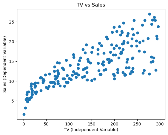
As you can see from the plot above, the relationship between TV and Sales is linear. As we increase the amount of money spent on TV advertising, the Sales also increases.
Now, if we have to predict the Sales based on the amount of money spent on TV advertising, we can use the above hypothesis. But we need to find the values of $\beta_0$ and $\beta_1$ to make the prediction. For that we will use the Linear Regression model.
Best Fit Line
The best fit line is the line that best fits the data points. We will use Ordinary Least Squares method to find the best fit line. The objective of Ordinary Least Squares (OLS) method is to minimize the sum of the squared differences between the actual values and the predicted values.
Residual
The difference between the actual value and the predicted value is called the residual. The sum of the squared residuals is called the Residual Sum of Squares (RSS). The objective of Ordinary Least Squares method is to minimize the RSS.
Residual = Actual Value - Predicted Value
$$ e_i = y_i - \hat{y_i} $$
Where,
- $e_i$ is the residual for the i-th data point
- $y_i$ is the actual value for the i-th data point
- $\hat{y_i}$ is the predicted value for the i-th data point (value on the best fit line)
# Set the theme for the plot
sns.set_theme(style="whitegrid")
sns.set_context("paper")

# 10 random samples from the dataset
sample = df.sample(10, random_state=42).reset_index(drop=True)

# Select two values from the sample to define a simple line
point1 = sample.iloc[0]
point2 = sample.iloc[2]

# Get the coordinates of the two points
x1, y1 = point1['TV'], point1['Sales']
x2, y2 = point2['TV'], point2['Sales']

# Calculate the slope (a) and intercept (b) of the line
a = (y2 - y1) / (x2 - x1)
b = y1 - a * x1

# Calculate the predicted values using the simple line
sample['Predicted Sales'] = a * sample['TV'] + b

# Calculate the residuals (actual - predicted)
sample['Residuals'] = sample['Sales'] - sample['Predicted Sales']

# Plotting the sample
plt.figure(figsize=(10, 6))

# Scatter plot of actual sales
plt.scatter(sample['TV'], sample['Sales'], label='Actual Sales', color='peru')

# Plot the simple line based on the two selected points
plt.plot(sample['TV'], a * sample['TV'] + b, color='steelblue', label='Connecting Line')

# Scatter plot of predicted sales
plt.scatter(sample['TV'], sample['Predicted Sales'], label='Predicted Sales', marker='x', color='dodgerblue')

# Plot the residuals as vertical lines
for i, row in sample.iterrows():
    plt.plot((row['TV'], row['TV']), (row['Sales'], row['Predicted Sales']), color='coral', linestyle='dotted')

# Adding labels and title
plt.xlabel('TV Advertising Budget')
plt.ylabel('Sales')
plt.title('Scatter Plot with Residuals and Connecting Line')

# Adding a legend to the plot
plt.legend()

# Adding grid for better readability
plt.grid(True)

# Show the plot
plt.show()

# Slope and intercept of the connecting line of two random points
print(f'Slope (a): {a:.2f}')
print(f'Intercept (b): {b:.2f}')

# Display the sample with residuals
sample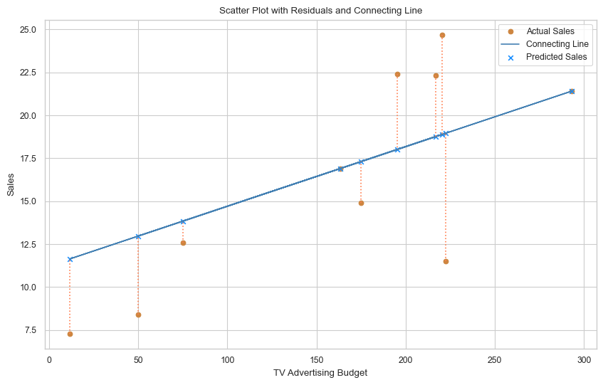
Slope (a): 0.03
Intercept (b): 11.23
| TV | Sales | Predicted Sales | Residuals | |
|---|---|---|---|---|
| 0 | 163.3 | 16.9 | 16.900000 | 0.000000 |
| 1 | 195.4 | 22.4 | 18.014583 | 4.385417 |
| 2 | 292.9 | 21.4 | 21.400000 | 0.000000 |
| 3 | 11.7 | 7.3 | 11.636111 | -4.336111 |
| 4 | 220.3 | 24.7 | 18.879167 | 5.820833 |
| 5 | 75.1 | 12.6 | 13.837500 | -1.237500 |
| 6 | 216.8 | 22.3 | 18.757639 | 3.542361 |
| 7 | 50.0 | 8.4 | 12.965972 | -4.565972 |
| 8 | 222.4 | 11.5 | 18.952083 | -7.452083 |
| 9 | 175.1 | 14.9 | 17.309722 | -2.409722 |
In above plot we have took 10 random samples from our dataset. And created a scatter plot of Actual Sales vs TV advertising. Then we took 2 points and created a line between them. This line is our best fit line till now. But this line is not the best fit line. We need to find the best fit line which will minimize the sum of squared residuals.
The sum of squared residuals is given by:
$$ RSS = \sum_{i=1}^{n} e_i^2 $$
Where,
- n is the number of data points
- $e_i$ is the residual for the i-th data point
We square the residuals to make them positive and then sum them up. From the table above you can see that residuals can be positive or negative. If we don’t square the residuals, the positive and negative residuals will cancel each other out and the sum of residuals will be zero. So, we square the residuals to make them positive and then sum them up to get the Residual Sum of Squares (RSS).
Ordinary Least Squares (OLS)
The objective of Ordinary Least Squares method is to minimize the Residual Sum of Squares (RSS). We do this by finding the values of $\beta_0$ and $\beta_1$ that minimize the RSS.
The formula to calculate the coefficients $\beta_0$ and $\beta_1$ is given by:
$$ \beta_1 = \frac{\sum_{i=1}^{n} (x_i - \bar{x})(y_i - \bar{y})}{\sum_{i=1}^{n} (x_i - \bar{x})^2} $$
$$ \beta_0 = \bar{y} - \beta_1 * \bar{x} $$
Where,
- n is the number of data points
- $x_i$ is the value of the independent variable for the i-th data point
- $y_i$ is the value of the dependent variable for the i-th data point
- $\bar{x}$ is the mean of the independent variable
- $\bar{y}$ is the mean of the dependent variable
The formula to calculate the coefficients $\beta_0$ and $\beta_1$ is given by:
| $TV (x_i)$ | $Sales (y_i)$ | $(x_i - \bar{x})$ | $(y_i - \bar{y})$ | $(x_i - \bar{x}) * (y_i - \bar{y})$ | $(x_i - \bar{x})^2$ | |
|---|---|---|---|---|---|---|
| 0 | 163.3 | 16.9 | 1 | 0.66 | 0.66 | 1 |
| 1 | 195.4 | 22.4 | 33.1 | 6.16 | 203.896 | 1095.61 |
| 2 | 292.9 | 21.4 | 130.6 | 5.16 | 673.896 | 17056.36 |
| 3 | 11.7 | 7.3 | -150.6 | -8.94 | 1346.364 | 22680.36 |
| 4 | 220.3 | 24.7 | 58 | 8.46 | 490.68 | 3364 |
| 5 | 75.1 | 12.6 | -87.2 | -3.64 | 317.408 | 7603.84 |
| 6 | 216.8 | 22.3 | 54.5 | 6.06 | 330.27 | 2970.25 |
| 7 | 50 | 8.4 | -112.3 | -7.84 | 880.432 | 12611.29 |
| 8 | 222.4 | 11.5 | 60.1 | -4.74 | -284.874 | 3612.01 |
| 9 | 175.1 | 14.9 | 12.8 | -1.34 | -17.152 | 163.84 |
| Mean | 162.3 | 16.24 | Sum | 3941.58 | 71158.56 |
$$ \beta_1 = \frac{\sum_{i=1}^{n} (x_i - \bar{x})(y_i - \bar{y})}{\sum_{i=1}^{n} (x_i - \bar{x})^2} = \frac{3941.58}{71158.56} = 0.0554 $$
$$ \beta_0 = \bar{y} - \beta_1 * \bar{x} = 16.24 - 0.0554 * 162.3 = 7.2500 $$
There is a simple way to calculate the coefficients $\beta_0$ and $\beta_1$ using the LinearRegression class from the sklearn.linear_model module. We will use this class to calculate the coefficients $\beta_0$ and $\beta_1$ for our example. First we will calculate the coefficients $\beta_0$ and $\beta_1$ of our sample data to check if we get the same values as calculated above. Then we will calculate the coefficients $\beta_0$ and $\beta_1$ of the entire dataset.
X = sample[['TV']].values
y = sample['Sales'].values
from sklearn.linear_model import LinearRegression
lr_model = LinearRegression()
lr_model.fit(X, y)
# Get the slope and intercept of the linear model
intercept = lr_model.intercept_
slope = lr_model.coef_[0]
print(f'The slope of the linear model is {slope:.2f}')
print(f'The intercept of the linear model is {intercept:.2f}')The slope of the linear model is 0.06
The intercept of the linear model is 7.25
As you can see from the results of linear regression model, our calculated values of $\beta_0$ and $\beta_1$ are same as the values calculated using the LinearRegression class. So, we have successfully calculated the coefficients $\beta_0$ and $\beta_1$ using the Ordinary Least Squares method.
Linear Regression Model
Now we will build the Linear Regression model using the all data points of the dataset. But first we will split the dataset into training and testing datasets. The usual practice is to split the dataset into 80% training data and 20% testing data.
We will use the training data to train our model and the testing data to predict the Sales from the TV advertising. We will then compare the predicted Sales with the actual Sales to evaluate the performance of our model.
# Split the dataset into training and testing sets
from sklearn.model_selection import train_test_split

# Independent variable (TV) and dependent variable (Sales)
X = df[['TV']]
y = df['Sales']

# Split the dataset into training and testing sets
X_train, X_test, y_train, y_test = train_test_split(X, y, test_size=0.2, random_state=42)

# Create a linear regression model
lr_model = LinearRegression()
lr_model.fit(X_train, y_train)

# Get the slope and intercept of the linear model
intercept = lr_model.intercept_
slope = lr_model.coef_[0]

print(f'The slope of the linear model is {slope:.2f}')
print(f'The intercept of the linear model is {intercept:.2f}')
The slope of the linear model is 0.05
The intercept of the linear model is 7.12
Therefore, the equation of the best fit line is given by:
$$ Sales = 7.12 + 0.05 * TV $$
Now we will use the Linear Regression model to predict the Sales based on the amount of money spent on TV advertising. We will use the testing data to make the prediction. We will then compare the predicted Sales with the actual Sales to evaluate the performance of our model.
# Predict the values using the model
y_pred = lr_model.predict(X_test)

# Calculate the residuals
residuals = y_test - y_pred

# Create a DataFrame to display the actual, predicted, and residuals
results = pd.DataFrame({'Actual': y_test, 'Predicted': y_pred, 'Residuals': residuals})
results.head()| Actual | Predicted | Residuals | |
|---|---|---|---|
| 96 | 16.9 | 14.717944 | 2.182056 |
| 16 | 22.4 | 16.211548 | 6.188452 |
| 31 | 21.4 | 20.748197 | 0.651803 |
| 159 | 7.3 | 7.664036 | -0.364036 |
| 129 | 24.7 | 17.370139 | 7.329861 |
Evaluation Metrics
There are several evaluation metrics to evaluate the performance of a regression model. Some of the common evaluation metrics are:
- Mean Squared Error (MSE) = $\frac{1}{n} \sum_{i=1}^{n} (y_i - \hat{y_i})^2$
- Root Mean Squared Error (RMSE) = $\sqrt{MSE}$
- R-squared (R2) = $1 - \frac{\sum_{i=1}^{n} (y_i - \hat{y_i})^2}{\sum_{i=1}^{n} (y_i - \bar{y})^2}$
Where,
Higher the R-squared value, better the model. The R-squared value lies between 0 and 1. A value closer to 1 indicates that the model is able to predict the values accurately. A value closer to 0 indicates that the model is not able to predict the values accurately.
We will cover these evaluation metrics in detail in the another blog.
For now, we will use them to evaluate the performance of our Linear Regression model.
# Evaluate the model using metrics
from sklearn.metrics import mean_squared_error, r2_score

# Calculate the Mean Squared Error (MSE)
mse = mean_squared_error(y_test, y_pred)

# Calculate the Root Mean Squared Error (RMSE)
rmse = np.sqrt(mse)

# Calculate the Coefficient of Determination (R^2)
r2 = r2_score(y_test, y_pred)

print(f'Mean Squared Error (MSE): {mse:.2f}')
print(f'Root Mean Squared Error (RMSE): {rmse:.2f}')
print(f'R^2 Score: {r2:.2f}')
Mean Squared Error (MSE): 10.20
Root Mean Squared Error (RMSE): 3.19
R^2 Score: 0.68
Our Linear Regression model has an R-squared value of 0.68. This means that our model is able to predict the Sales accurately 68% of the time.
Actual vs Predicted Sales
We will plot the Actual Sales vs Predicted Sales to visualize how well our model is able to predict the Sales based on the amount of money spent on TV advertising.
# Plot the actual vs predicted values
plt.figure(figsize=(10, 6))

# Scatter plot of actual vs predicted values
plt.scatter(y_test, y_pred, color='coral')

# Plot a line
plt.plot([y_test.min(), y_test.max()], [y_test.min(), y_test.max()], color='steelblue')

# Adding labels and title
plt.xlabel('Actual Sales')
plt.ylabel('Predicted Sales')
plt.title('Actual vs Predicted Sales')
plt.grid(True)
plt.show()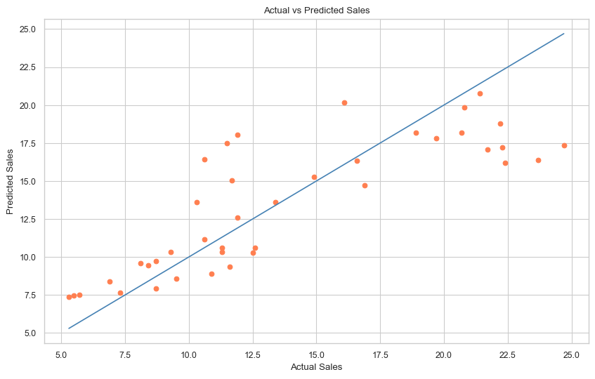
Elements of the plot
In the plot above,
- Orange dots represents a pair of actual sales (
y_test) and predicted sales (y_pred). - The blue line represents the line where actual sales is equal to predicted sales.
- The closer the orange dots are to the blue line, the better the model is able to predict the sales.
Interpretation of the plot
We can see from the plot that our linear regression model captures the general trend, but the deviation is higher for higher values of Sales.
As our model is very simple and we only have one independent variable, the model is not able to capture all the patterns in the data. Using more variables will help us to build a better model.
Plotting the Regression Line using Model
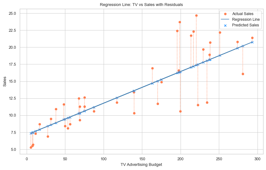
We will plot the regression line using the predicted values of Sales. The regression line is the line that best fits the data points.
# Reset the index of X_test and y_test to align with y_pred
X_test.reset_index(drop=True, inplace=True)
y_test.reset_index(drop=True, inplace=True)

# Plot the regression line using model's coefficient and intercept
plt.figure(figsize=(10, 6))
plt.scatter(X_test['TV'], y_test, color='coral', label='Actual Sales')

# Plot the regression line using the predicted values
plt.plot(X_test['TV'], y_pred, color='steelblue', label='Regression Line')

# Scatter plot of predicted sales
plt.scatter(X_test['TV'], y_pred, label='Predicted Sales', marker='x', color='dodgerblue')

# Plot the residuals as vertical lines
for i, row in X_test.iterrows():
    plt.plot((row['TV'], row['TV']), (y_pred[i], y_test.loc[i]), color='coral', linestyle='dotted')

# Adding labels and title
plt.xlabel('TV Advertising Budget')
plt.ylabel('Sales')
plt.title('Regression Line: TV vs Sales with Residuals')
plt.legend()
plt.grid(True)
plt.show()
Elements of the plot
In the plot above,
- The orange dots represent the actual sales values.
- The blue x’s represent the predicted sales values.
- The blue line represents the regression line.
- The orange dotted line represents the residuals (difference between actual sales and predicted sales).
Interpretation of the plot
- The regression line shows a positive slope, indicating that the model has learned that an increase in TV advertising budget is generally associated with an increase in Sales.
- The orange dots (actual sales) that are close to the regression line (predicted sales) indicate that the model is able to predict the sales accurately.
- The orange dots (actual sales) that are far from the regression line (predicted sales) indicate that the model is not able to predict the sales accurately.
- The errors (residuals) appears to be more spread out at higher TV advertising budgets, indicating that the model is not able to predict the sales accurately for higher TV advertising budgets.
Conclusion
In this blog post, we explored the relationship between TV advertising budgets and sales using simple linear regression. Through the visualizing the data, we observed a positive linear relationship between TV advertising budgets and sales.
We then built a simple linear regression model to predict the sales based on the amount of money spent on TV advertising. We calculated the coefficients $\beta_0$ and $\beta_1$ using the Ordinary Least Squares method. We then used the Linear Regression model to predict the sales based on the amount of money spent on TV advertising.
The model has an R-squared value of 0.68, indicating that the model is able to predict the sales accurately 68% of the time. The model captures the general trend, but the deviation is higher for higher values of Sales. Using more variables will help us to build a better model.
In the next blog post, we will explore multiple linear regression, where we will use more than one independent variable to predict the dependent variable.
Deployment
The simple linear regression model has been deployed to predict sales revenue based on individual advertising budgets for TV, Radio, and Newspaper. Seperate models have been built for each advertising medium. The model can be accessed at the following links: Simple Linear Regression
← Back to Blog