Binary Classification of Insurance Cross Selling

Sep 11, 2024

Overview

In this challenge, I tackle the problem of binary classification for insurance cross-selling. The task involves predicting whether an existing insurance customer will purchase an additional product based on various customer attributes. This is part of my 30 Kaggle Challenges in 30 Days series.

Problem Description

The dataset consists of customer information, and the goal is to predict whether each customer will purchase a new insurance product. This is a classic binary classification problem with two possible outcomes:

1: The customer buys the additional insurance.
0: The customer does not buy the additional insurance.

Approach

1. Exploratory Data Analysis (EDA)

I analyse the dataset to uncover patterns, correlations, and missing data. Key EDA steps include:

   id  Gender  Age  Driving_License  Region_Code  Previously_Insured  \
0   0    Male   21                1         35.0                   0   
1   1    Male   43                1         28.0                   0   
2   2  Female   25                1         14.0                   1   
3   3  Female   35                1          1.0                   0   
4   4  Female   36                1         15.0                   1   

  Vehicle_Age Vehicle_Damage  Annual_Premium  Policy_Sales_Channel  Vintage  \
0    1-2 Year            Yes         65101.0                 124.0      187   
1   > 2 Years            Yes         58911.0                  26.0      288   
2    < 1 Year             No         38043.0                 152.0      254   
3    1-2 Year            Yes          2630.0                 156.0       76   
4    1-2 Year             No         31951.0                 152.0      294   

   Response  
0         0  
1         1  
2         0  
3         0  
4         0

We have 5 numerical features and 5 categorical features.
Numerical Features: Age, Region Code, Annual Premium, Policy Sales Channel, and Vintage
Categorical Features: Gender, Driving License, Previously Insured, Vehicle Age, and Vehicle Damage

Missing Data

train.isnull().sum()

id                      0
Gender                  0
Age                     0
Driving_License         0
Region_Code             0
Previously_Insured      0
Vehicle_Age             0
Vehicle_Damage          0
Annual_Premium          0
Policy_Sales_Channel    0
Vintage                 0
Response                0
dtype: int64

Training data don’t have any missing data.

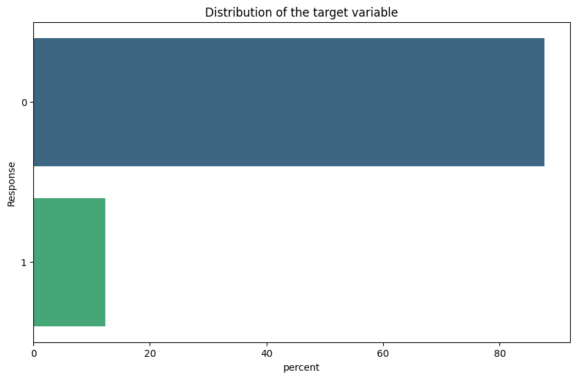
Distribution of Target Variable

plt.figure(figsize=(10, 6))
sns.countplot(train, y='Response', stat='percent', hue='Response', palette='viridis', legend=False)
plt.title('Distribution of the target variable')
plt.show()

Distribution of the target variable for Kaggle Playground Series S4E7 competition

87.7% of the customers have not purchased insurance, and 12.3% have purchased insurance. The data is highly imbalanced.

Other Features

Only 4.14% of the vehicles are older than 2 years.
The Annual Premium feature contains 18.36% lower and 2.3% upper outliers.

2. Feature Engineering

To improve the model’s accuracy, we need to perform feature engineering.

Encoding Categorical Features

We will do one hot encoding of categorical features because machine learning models need numerical values.

# One-hot encode the categorical columns
ohe = OneHotEncoder()
X_train_cat = ohe.fit_transform(X_train[cat_cols]).toarray()
X_test_cat = ohe.transform(X_test[cat_cols]).toarray()

Scaling Numerical Features

We will scale the numerical features so that all the features are on the same scale.

# Standardize the numerical columns
ss = StandardScaler()
X_train_num = ss.fit_transform(X_train[num_cols])
X_test_num = ss.transform(X_test[num_cols])

Now, we will merge both the encoded and scaled data.

# Combine the numerical and categorical columns
X_train = np.hstack((X_train_num, X_train_cat))
X_test = np.hstack((X_test_num, X_test_cat))

3. Model Selection

For this binary classification task, I experiment with several machine-learning models.
I created five folds of data using stratified k folds to validate the results before building a final model for submission. By doing this, we minimized the effect of imbalanced data. So each model will be run on five different combinations of the same data, except the random forest classifier. Because it was taking too much time, I have only one fold result for it.

Logistic Regression

A simple but effective model for binary classification.

Results:

Fold=0, AUC=0.8415943240518661
Fold=1, AUC=0.8413122123292518
Fold=2, AUC=0.8412833425884464
Fold=3, AUC=0.8408804706148243
Fold=4, AUC=0.8414265096586687

Random Forest

A powerful ensemble method that handles feature interactions well. Random Forest tends to be more computationally expensive as it grows and averages multiple decision trees.

Results:

Fold=0, AUC=0.8444239686596572

XGBoost

A high-performance model for classification tasks optimized for speed and accuracy.

Results:

Fold=0, AUC=0.8778452687486167
Fold=1, AUC=0.8779387120291394
Fold=2, AUC=0.8782061206725237
Fold=3, AUC=0.8778056660814351
Fold=4, AUC=0.8786452067898584

Results

After experimenting with various methods, here are the best results achieved for this challenge:

Model Chosen: XGBoost
ROC-AUC: 0.87820

Key Learnings

XGBoost is better than logistic regression and random forest.
The random forest classifier is resource intensive and takes 10 minutes to run single-fold.
I tried to optimize the hyperparameter using RandomizedSearchCV, but my laptop ran out of memory and restarted after 35 minutes.

Future Improvements

While the initial analysis focuses on traditional models like logistic regression, random forest, and XGBoost, there are several advanced techniques I plan to explore in the future to further improve performance:

Deep Learning Model: Experimenting with neural networks to capture more complex patterns in the data.
Ensemble Models: Using advanced stacking techniques that combine the predictions of multiple models for higher accuracy.
AutoML: Leveraging automated machine learning frameworks to optimize the selection and tuning of models.
Feature Selection: Investigating more sophisticated feature selection methods, such as Recursive Feature Elimination(RFE), to improve model efficiency.

This section will be updated as I explore new techniques and models, providing a comparison with the initial results.

Conclusion

The first day of the 30 Kaggle Challenges in 30 Days journey has been both challenging and insightful, especially while experimenting with various binary classification models. After browsing some discussions on the Kaggle website, I realized there is so much more to learn. Hopefully, this challenge will increase my knowledge of machine learning. I am looking forward to completing the rest of the 29 days.

For those interested in the complete code and implementation details, feel free to check out the GitHub repository.

← Back to Blog