Classification with an Academic Success Dataset
Sep 12, 2024
Overview
This is the second challenge of the 30 Kaggle Challenges in 30 Days series. Yesterday, we worked on a binary classification for insurance cross-selling, and today, we are tackling a multiclass classification problem to predict students’ academic outcomes.
Kaggle Season 4 Episode 6
The dataset for this competition was generated from a deep learning model trained on the Predict Students’ Dropout and Academic Success dataset. The features are close to, but not exactly the same as, the original. Our task is to build a multiclassification model to predict students’ dropout and academic success.
This is a 3-category classification problem with a notable imbalance between classes.
Exploratory Data Analysis (EDA)
Dataset Overview
train = pd.read_csv(train.csv)
train.shape
(76518, 38)
The train dataset has 76518 rows and 38 columns. Next, we will check the value counts of the target variable. Before that, you can check the head to get an idea of the various columns. But this dataset has so many columns that I can’t write them here (it won’t look good).
train.Target.value_counts()Target
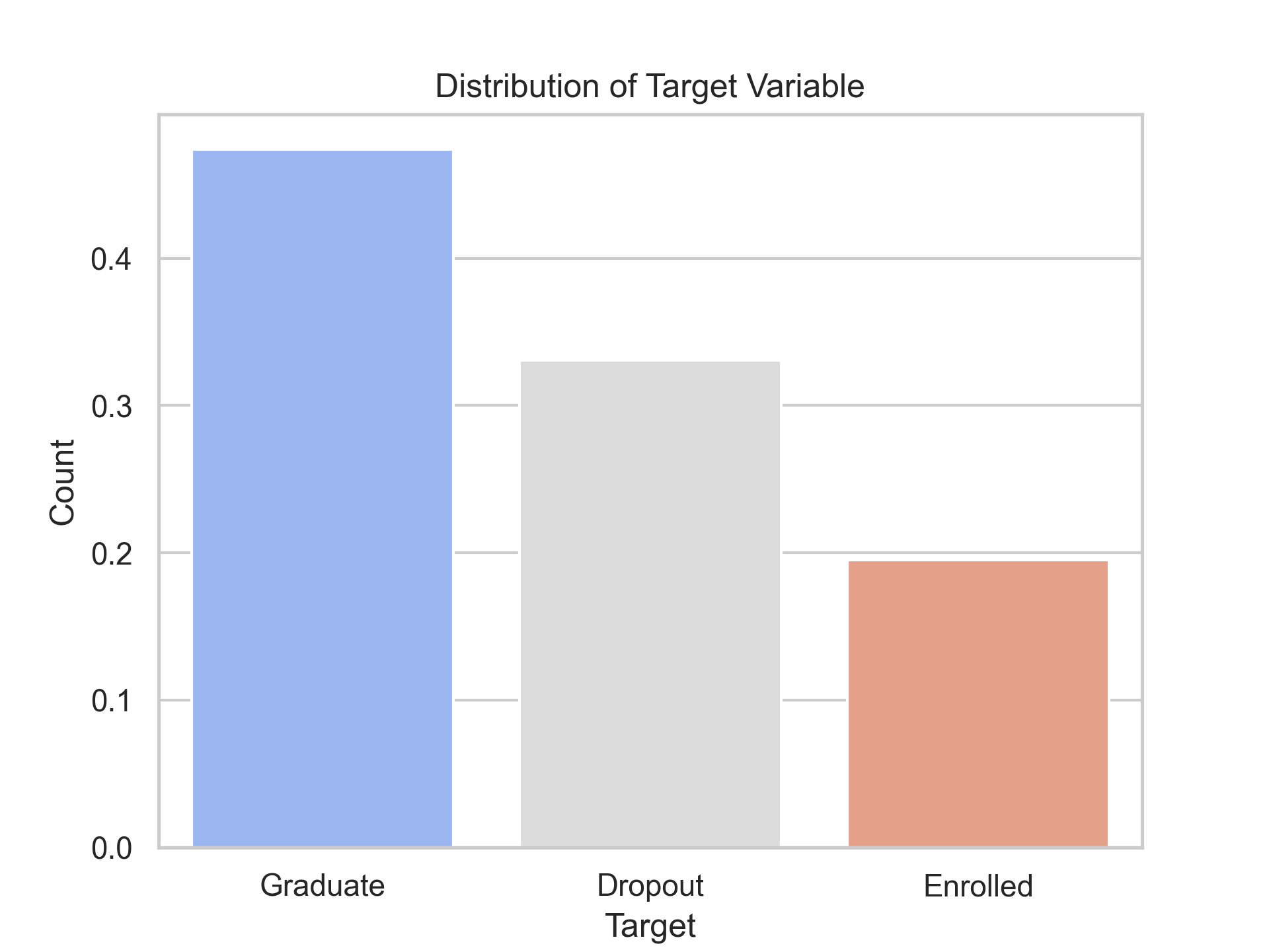
Graduate 36282
Dropout 25296
Enrolled 14940
Name: count, dtype: int64
From the plot, you can see that the majority of the students graduated, 33% dropped out, and the rest enrolled. There is an imbalance in the target feature. As the evaluation metric is accuracy, having imbalanced data can give us a wrong idea about the perfection of our model. We will need to handle the data imbalance to make good predictions in all categories.
Missing Values
Checked for missing values. Train dataset don’t have any missing values.
train.isna().sum()id 0
Marital status 0
Application mode 0
Application order 0
Course 0
Daytime/evening attendance 0
Previous qualification 0
Previous qualification (grade) 0
Nacionality 0
Mother's qualification 0
Father's qualification 0
Mother's occupation 0
Father's occupation 0
Admission grade 0
Displaced 0
Educational special needs 0
Debtor 0
Tuition fees up to date 0
Gender 0
Scholarship holder 0
Age at enrollment 0
International 0
Curricular units 1st sem (credited) 0
Curricular units 1st sem (enrolled) 0
Curricular units 1st sem (evaluations) 0
Curricular units 1st sem (approved) 0
Curricular units 1st sem (grade) 0
Curricular units 1st sem (without evaluations) 0
Curricular units 2nd sem (credited) 0
Curricular units 2nd sem (enrolled) 0
Curricular units 2nd sem (evaluations) 0
Curricular units 2nd sem (approved) 0
Curricular units 2nd sem (grade) 0
Curricular units 2nd sem (without evaluations) 0
Unemployment rate 0
Inflation rate 0
GDP 0
Target 0
dtype: int64Data Types
Check the datatypes of the features.
train.info()<class 'pandas.core.frame.DataFrame'>
RangeIndex: 76518 entries, 0 to 76517
Data columns (total 38 columns):
# Column Non-Null Count Dtype
--- ------ -------------- -----
0 id 76518 non-null int64
1 Marital status 76518 non-null int64
2 Application mode 76518 non-null int64
3 Application order 76518 non-null int64
4 Course 76518 non-null int64
5 Daytime/evening attendance 76518 non-null int64
6 Previous qualification 76518 non-null int64
7 Previous qualification (grade) 76518 non-null float64
8 Nacionality 76518 non-null int64
9 Mother's qualification 76518 non-null int64
10 Father's qualification 76518 non-null int64
11 Mother's occupation 76518 non-null int64
12 Father's occupation 76518 non-null int64
13 Admission grade 76518 non-null float64
14 Displaced 76518 non-null int64
15 Educational special needs 76518 non-null int64
16 Debtor 76518 non-null int64
17 Tuition fees up to date 76518 non-null int64
18 Gender 76518 non-null int64
19 Scholarship holder 76518 non-null int64
20 Age at enrollment 76518 non-null int64
21 International 76518 non-null int64
22 Curricular units 1st sem (credited) 76518 non-null int64
23 Curricular units 1st sem (enrolled) 76518 non-null int64
24 Curricular units 1st sem (evaluations) 76518 non-null int64
25 Curricular units 1st sem (approved) 76518 non-null int64
26 Curricular units 1st sem (grade) 76518 non-null float64
27 Curricular units 1st sem (without evaluations) 76518 non-null int64
28 Curricular units 2nd sem (credited) 76518 non-null int64
29 Curricular units 2nd sem (enrolled) 76518 non-null int64
30 Curricular units 2nd sem (evaluations) 76518 non-null int64
31 Curricular units 2nd sem (approved) 76518 non-null int64
32 Curricular units 2nd sem (grade) 76518 non-null float64
33 Curricular units 2nd sem (without evaluations) 76518 non-null int64
34 Unemployment rate 76518 non-null float64
35 Inflation rate 76518 non-null float64
36 GDP 76518 non-null float64
37 Target 76518 non-null object
dtypes: float64(7), int64(30), object(1)
memory usage: 22.2+ MBAs you can see, all of the features except the target feature are numerical. The reason for this is that all of the data is already encoded. Features like Marital status, Application mode, Course, etc. are categorical data originally and the description is available at UCI ML Repository.
First, we will use the data directly in the numerical form provided by Kaggle. Later, we can convert the data into its categorical form to do feature engineering.
Our main goal is to build an ML model, so I am not going to do detailed data analysis. However, it would be helpful if we were required to do feature engineering. I have prepared plots and detailed statistics on each feature in jupyter notebook in case you are interested in going through it.
Handling Imbalance with Stratified K-Fold Cross-Validation
The next task is to create a stratified K-fold cross-validation from the training set to validate the models before building the final model. By validating the models on different folds, we can gain insights into how well the model will perform on unseen data. Since the target variable is highly imbalanced, using a stratified K-fold ensures that each fold maintains the same proportion of the target variable as in the original dataset.
import pandas as pd
from sklearn.model_selection import StratifiedKFold

def create_fold(fold):
    # import data
    data = pd.read_csv('./input/train.csv')
    data['kfold'] = -1
    data = data.sample(frac=1).reset_index(drop=True)
    y = data.Target.values
    skf = StratifiedKFold(n_splits=fold)
    for f, (t_, v_) in enumerate(skf.split(X=data, y=y)):
        data.loc[v_, 'kfold'] = f
    data.to_csv('./input/train_folds.csv', index=False)

if __name__ == '__main__':
    create_fold(5)
Feature Scaling
Scaling the numerical features. Since all the features have numerical data type, we will scale all features.
# Initialize the StandardScaler
scaler = StandardScaler()

# Fit and transform the training data
X_train = scaler.fit_transform(X_train)
X_test = scaler.transform(X_test)
Model Training and Evaluation
We will not try different models and evaluate their performance. The evaluation metric is accuracy.
Logistic Regression
from sklearn.linear_model import LogisticRegressionResults:
Fold=0, Accuracy=0.8187401986408782
Fold=1, Accuracy=0.814231573444851
Fold=2, Accuracy=0.8159958180867747
Fold=3, Accuracy=0.8163105273475789
Fold=4, Accuracy=0.8166372606678429
Decision Tree Classifier
from sklearn.tree import DecisionTreeClassifierResults:
Fold=0, Accuracy=0.7449032932566649
Fold=1, Accuracy=0.7400679560899112
Fold=2, Accuracy=0.7374542603240982
Fold=3, Accuracy=0.7370450238515324
Fold=4, Accuracy=0.7412925570149644
Random Forest Classifier
from sklearn.ensemble import RandomForestClassifierResults:
Fold=0, Accuracy=0.8278881338212232
Fold=1, Accuracy=0.8227914270778881
Fold=2, Accuracy=0.8259278619968635
Fold=3, Accuracy=0.8231719270731229
Fold=4, Accuracy=0.8272887669084493
SVM
from sklearn.svm import SVCResults:
Fold=0, Accuracy=0.8208311552535285
Fold=1, Accuracy=0.8147543125980136
Fold=2, Accuracy=0.8207004704652379
Fold=3, Accuracy=0.8194471672221133
Fold=4, Accuracy=0.8220610337842253
Gradient Boosting Classifier
from sklearn.ensemble import GradientBoostingClassifierResults:
Fold=0, Accuracy=0.8295216936748563
Fold=1, Accuracy=0.8273000522739153
Fold=2, Accuracy=0.8282148457919498
Fold=3, Accuracy=0.8248709403384957
Fold=4, Accuracy=0.8280729268770829
XGBoost Classifier
from xgboost import XGBClassifierResults:
Fold=0, Accuracy=0.8325927861996864
Fold=1, Accuracy=0.8284762153685311
Fold=2, Accuracy=0.8296523784631469
Fold=3, Accuracy=0.8267006469319741
Fold=4, Accuracy=0.8330392733450958
Model Comparison
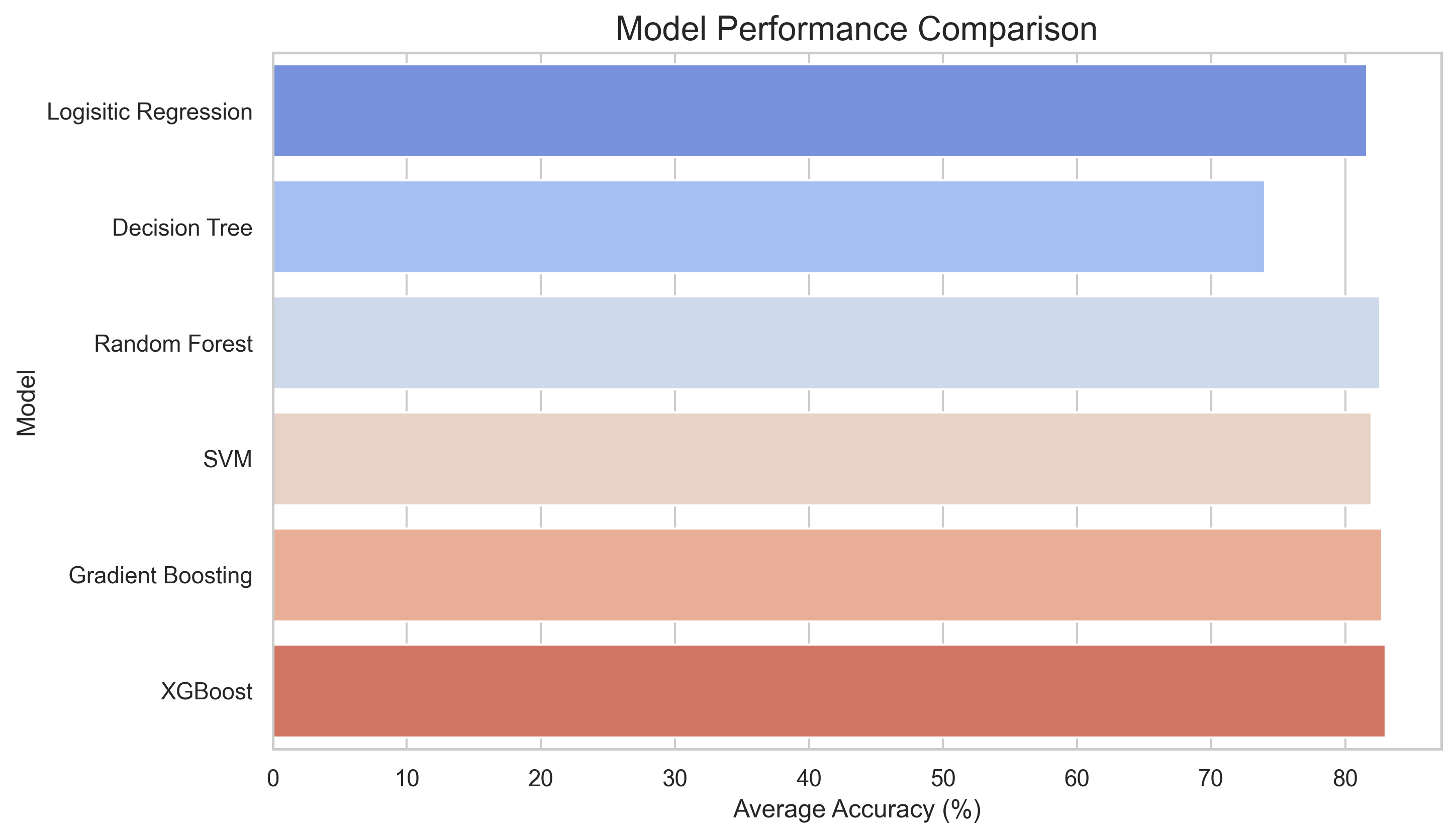
Here’s a comparison of the models tested:

| Model | Average Accuracy |
|---|---|
| Logistic Regression | 81.64% |
| Decision Tree Classifier | 74.01% |
| Random Forest Classifier | 82.59% |
| SVM | 81.96% |
| Gradient Boosting | 82.76% |
| XGBoost | 83.01% |
XGBoost gave us the best results, making it the model of choice for final submission.
Final Model and Submission
We have selected the XGBoost for our final submission. After training on the entire dataset, we achieved a final accuracy score of 83.45%.
You can check the code in Kaggle Notebook.
Key Learnings
- Label Encoding for XGBoost: XGBoost does not accept string values in the target variable, so I had to label encode the target values.
- Automated Model Testing: I have implemented a command-line script to automate the running of multiple models using different folds. This allows me to efficiently test various models, streamlining the experimentation process. I will write a detailed blog on this topic, so stay tuned. For now, you can check the code in the GitHub repository.
Conclusion
This was the second day of the 30 Kaggle Challenges in 30 Days series, and we successfully completed a multiclass classification problem. Feel free to try the code from Kaggle Notebook and share your result!
← Back to Blog