Regression with an Abalone Dataset

Sep 14, 2024

Overview

Today is the fourth day of 30 Kaggle Challenges in 30 Days. In the last three challenges, I concentrated on basic models and building a basic pipeline for the Kaggle competition. Today, I will deep-dive into other areas, like feature engineering or hyperparameter tuning, to optimize the model’s performance.

Problem Description

Today, we are solving the Kaggle Playground Season 4 Episode 4 problem. The dataset for this problem is synthetically generated by using the dataset from the UC Irvine Machine Learning Repository. Links for both are given below:

Kaggle Playground: Season 4, Episode 4
Abalone Dataset on UCI: Original Dataset

In this problem, we have to build a model to predict the age of an abalone from physical measurements. The evaluation metric for this competition is Root Mean Squared Logarithmic Error.

Data Exploration

Train Data: 90615 rows and 9 columns
Test Data: 60411 rows and 8 columns

The train data have one more column because it contains the target feature, Rings. You may wonder that our target must be age, so why does the train dataset have the target feature Rings? Well, in the original dataset, you calculate age by adding 1.5 to the number of rings, and the same goes here as well.

Missing Values

The train dataset doesn’t have any missing values. All features except Sex are numerical. The number of unique values for each of the features is given below:

Sex                  3
Length             157
Diameter           126
Height              90
Whole weight      3175
Whole weight.1    1799
Whole weight.2     979
Shell weight      1129
Rings               28

The following is the variable table from the source. Kaggle has replaced Shucked_weight with Whole weight.1 and Viscera_weight with Whole weight.2.

Variable Name	Role	Type	Description	Units	Missing Values
Sex	Feature	Categorical	M, F, and I (infant)		no
Length	Feature	Continuous	Longest shell measurement	mm	no
Diameter	Feature	Continuous	Perpendicular to length	mm	no
Height	Feature	Continuous	With meat in shell	mm	no
Whole_weight	Feature	Continuous	Whole abalone	grams	no
Shucked_weight	Feature	Continuous	Weight of meat	grams	no
Viscera_weight	Feature	Continuous	Gut weight (after bleeding)	grams	no
Shell_weight	Feature	Continuous	After being dried	grams	no
Rings	Target	Integer	+1.5 gives the age in years		no

I got this pictures from flickr and dimension website to understand the dimension.

Abalone

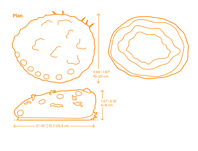
Target Feature: Rings

The rings are used to calculate age. The age of an abalone is determined by cutting the shell through the cone, staining it, and counting the number of rings through a microscope—a boring and time-consuming task, according to the researchers who collected data for this project.

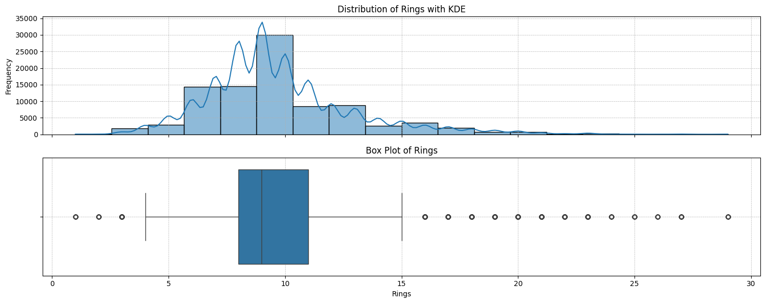
Distribution of Kaggle S4E4 Target Variable (Rings)

From the plot, we can see that there are some outliers. The median rings are 9, and most of the abalone have rings between 8 and 11.

Pipeline

Today, I tried using the pipeline to run all the preprocessing. Pipelines in scikit-learn help streamline the process by handling preprocessing and model training in one step, ensuring that all folds receive the same transformations and making the code modular and reusable.

In our dataset, we have only one categorical variable, Sex, which I encoded using OneHotEncoder. The rest of the features are numerical features, which I scaled using the standard scaler from Sklearn.


def run(fold, model):
    # Import the data
    df = pd.read_csv(config.TRAINING_FILE)

    # Split the data into training and testing
    train = df[df.kfold != fold].reset_index(drop=True)
    test = df[df.kfold == fold].reset_index(drop=True)

    # Split the data into features and target
    X_train = train.drop(['id', 'Rings', 'kfold'], axis=1)
    X_test = test.drop(['id', 'Rings', 'kfold'], axis=1)

    y_train = train.Rings.values
    y_test = test.Rings.values

    # Define categorical and numerical columns
    categorical_cols = ['Sex']
    numerical_cols = [col for col in X_train.columns if col not in categorical_cols]

    # Create a column transformer for one-hot encoding and standard scaling
    preprocessor = ColumnTransformer(
        transformers=[
            ('num', StandardScaler(), numerical_cols),
            ('cat', OneHotEncoder(drop='first'), categorical_cols)
        ]
    )

    # Create a pipeline with the preprocessor and the model
    pipeline = Pipeline(steps=[
        ('preprocessor', preprocessor),
        ('model', model_dispatcher.models[model])
    ])

	# Fit the model
	pipeline.fit(X_train, y_train)

	# make predictions
	preds = pipeline.predict(X_test)

	# Clip predictions to avoid negative values
	preds = np.clip(preds, 0, None)

	end = time.time()
	time_taken = end - start

	# Calculate the R2 score
	rmsle = root_mean_squared_log_error(y_test, preds)
	print(f"Fold={fold}, rmsle={rmsle:.4f}, Time={time_taken:.2f}sec")

Analysis of Results (RMSLE and Time Taken):

I have built five cross-validation sets to validate the model. I used a total of 10 models and fit them on every validation set. The results are as follows:

Model	Fold 0 RMSLE	Fold 1 RMSLE	Fold 2 RMSLE	Fold 3 RMSLE	Fold 4 RMSLE	Avg RMSLE	Avg Time (seconds)
Linear Regression	0.1646	0.1648	0.1662	0.1665	0.1627	0.1649	0.05
Random Forest	0.1552	0.1543	0.1558	0.1547	0.1536	0.1547	3.91
XGBoost	0.1512	0.1506	0.1526	0.1508	0.1498	0.1510	0.37
LightGBM	0.1505	0.1500	0.1518	0.1503	0.1494	0.1504	0.24
CatBoost	0.1497	0.1489	0.1506	0.1492	0.1483	0.1493	6.28
Gradient Boosting	0.1529	0.1529	0.1543	0.1527	0.1520	0.1530	6.59
SVR	0.1532	0.1535	0.1546	0.1535	0.1517	0.1533	253.64
KNeighbors Regressor	0.1658	0.1655	0.1671	0.1653	0.1646	0.1657	0.52
Ridge Regression	0.1646	0.1648	0.1662	0.1665	0.1627	0.1650	0.07
Lasso Regression	0.2161	0.2165	0.2177	0.2159	0.2160	0.2164	0.08

I got the best score from CatBoost without doing any feature engineering. The next best models are LightGBM and XGBoost, which also took very little time to run.

After this initial run, we have the following three options:

Hyperparameter Tuning: Using techniques like Grid Search, Randomized Search, and Bayesian Optimization (e.g., using Optuna).
Feature Engineering: Transformation, feature selection, creating new features.
Ensembling: Blending, Stacking, Bagging.

I will begin with hyperparameter tuning using Sklearn’s RandomizedGridSearchCV on CatBoost because that model achieves our best score.

Now, after running various grids for 3 hours, the score doesn’t improve. After multiple rounds of grid search and randomized search, the best RMSLE remained very similar to the default CatBoost model. This indicates that CatBoost’s default parameters are well-optimized for this dataset.

I should have begun with feature engineering, but for today, let’s finalize the CatBoost. I will explore the rest of the options for this problem in the future, and some I will use for tomorrow’s problem.

Final Result

I have used CatBoostRegressor on a full train set to build a model for submission and got the following result.

Model: CatBoost
Score: 0.14783
Rank Range: 1064-1069

Conclusion

Today was the fourth day of the challenge. I solved today’s problem using a pipeline. I tried to optimize the model using grid search, but it didn’t improve the performance. I spent around three hours doing that. Tomorrow, I will concentrate on feature engineering first after the initial stage of building base models.

Links

Notebook: Kaggle Notebook for S4E4
Code: GitHub Repository for Day 4

← Back to Blog